In this post, I’ll talk about some of the basics of logistic regression, and why we would use this type of modeling over linear regression. To help illustrate these concepts, I’ll use the Titanic dataset which can be found here.

Linear Model: Key Assumptions

Before we begin, let’s assume we want to use a linear regression model for our data, and keep in mind the key assumptions of a linear model:

• Linearity- our dependent and independent variables have a linear relationship
• Independence- the errors/residuals are independent
• Normality- the errors/residuals follow a normal distribution
• Equality of variances- the errors/residuals have generally equal variances/follow the same pattern

Example: Relationship between Age and Survival

Let’s take a simple example and check out survival based on age. The ‘Survived’ column is 0 for didn’t survive and 1 for did survive, and the age column is the passengers’ ages. We are wondering whether we can find a relationship between the age of the passenger and whether or not they survived. Here’s a scatter plot:

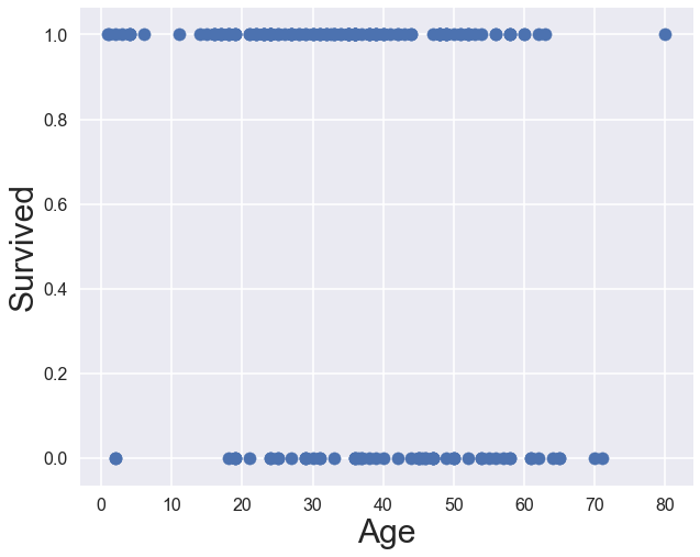
Notice how the points form two separate lines. If we think about what the ‘Survived’ variable is, it makes sense that we have two separate lines of points, as ‘Survived’ can only be either 0 or 1. How would we even place a line of best fit?

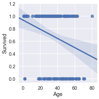
There isn’t an area that makes sense for a line to best describe the data we have. Referring back to the key assumptions, we can already cross off the linearity assumption: for X and Y to have a linear relationship, a change in 1 unit of X implies a change in Y. Our data doesn’t act in this condition, as one distinct age could be either of the Y values. While this data already doesn’t qualify for a linear model, we can confirm this by looking at the residuals.

import seaborn as sns
sns.residplot(x='Age',y='Survived', data=titanic)

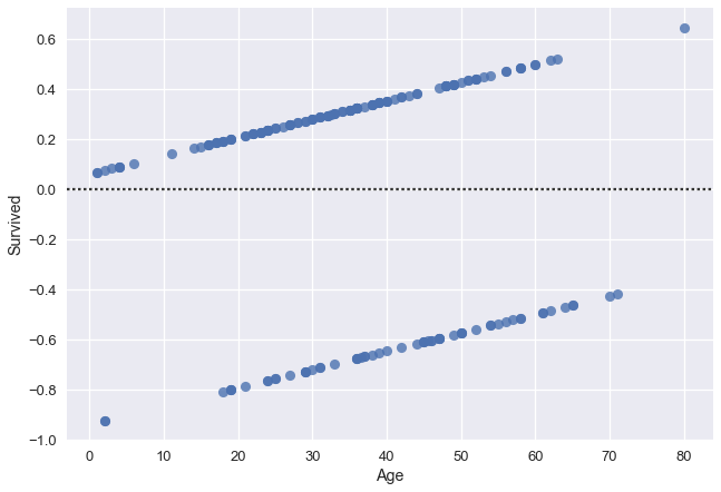Note- the residplot function above is extremely useful for determining whether or not a linear model can be used. You can check out the residuals without even having to fit the data to a linear regression model (function does that).

Clearly, we cannot say that the residuals follow a normal distribution. Why? A simple check is to observe the shape: a normal distribution is that of a bell curve, and we have parallel lines here. Two out of the four key assumptions do not apply to our data, and therefore, means we cannot use linear regression. Since we’ve proved this, moving forward we can just rule out linear regression for data where the dependent variable, ‘Survived’ in our case, has binary values.

Genearlized Linear Models

Before I go into why logistic regression is ideal for this scenario, I need to quickly discuss a Generalized Linear Model (GLM). There are three main characteristics of a GLM:

• Linear Component- relationship between X and y
• Link Component- transformation of linear regression line
• Random Component- error distribution

Linear Component

Instead of requiring a linear relationship between X and Y (linear regression), the standards are a bit more lax for a GLM–this is because we have a relationship between X and Y that isn’t linear, but we want to generalize this relationship into a linear relationship.

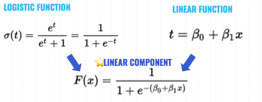
With respect to logistic regression, what is the linear component? Here is a little diagram showing how we take the log function and substitute in the equation of a line (linear equation). Basically, what’s happening is that the -t exponent in the denominator is replaced with the linear fcn, t. So the exponent becomes the right hand side of the linear equation:

Link Component

How do we get our link component? This link component links our linear component back to linear regression, and is called the logit. The logit is the inverse of the logistic function above.

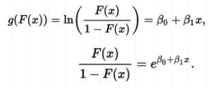
The second line here is simply specifying what we are taking the natural log of in the logit equation on the first line.

In this function, the betas are the coefficients, the log of the odds ratios. The exponentials are the odds ratios, or p/(1-p).

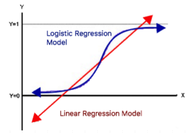
Check out the logit in comparison to a linear regression line:

Random Component

This is simply saying that the errors must be random, and Logistic Regression satisfies this as it has a binomial distribution.

Logistic Regression

Model Characteristics

• Generalized linear model
• Binary, mutually exclusive dependent variable
• Independent variables can be either categorical or numerical
• Models the probability that y = 1 given x values

Key Model Assumptions

• The independent variables are independent of one another
• The observations are independent of one another
• There is no measurement error in our observations
• The independent variables are linearly related to the log=odds that Y = 1

Final Details

Now for the main topic of this post: Logistic regression. Logistic regression is a non-linear model that requires a binary, mutually exclusive dependent variable. This can be either categorical or numerical. It takes a transformation of the linear equations (y=mx+b) to be able to Logistic regression is used to model the probability that our dependent variable is either 0 or 1. Additionally, instead of using the model to predict the value of the dependent variable based on our independent variable, logistic regression models predict the probability that our dependent variable will be 1. For all of these reasons, we can see how different the linear and logistic regression models are.

A bit more about the fit– we call our fit the logit (explained above), which you can compare to the best line of fit for a linear regression model. Our logit does not actually hit values 0 or 1, but approaches them closely. Another interpretation of this is that probability values fall between 0 and 1.